How to improve PostgreSQL performance? Try optimizing database and queries!

⚠️ WARNING: This article partially deals with Postgres server settings. About working with them, it’s necessary to understand that changing such settings can lead both to improvement and to deterioration of server performance.

Shared buffer

Postgresql uses two caches for his work, first of them is a shared buffer - native PSQL cache working by Clock Sweeo Angry principle. The second one is the OS cache - an operating system cache. Mostly OS cache works by principle of the Least Recent algorithm.

‍

The main advantage of a shared buffer is that in spite of the OS cache he is able to define which data is used the most often and keep them in memory much longer, he has a popularity score from 1 to 5. Then higher the score is, then faster data will be removed from buffer. That's why queries which go through a shared buffer are always better served.

‍

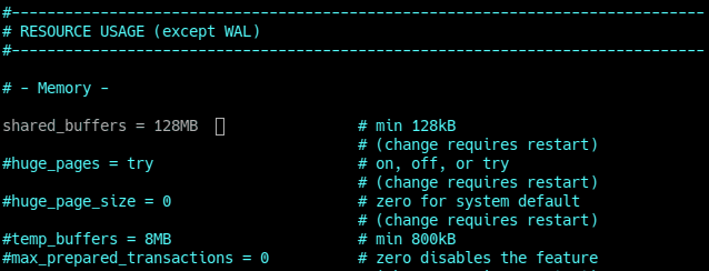
The main problem of the shared buffer is that it’s optimized only for server could start at the system with low settings. The default value for shared buffer in postgresql.conf is 128mb (param. name is shared_buffer) It’s supposed to be one of the harders params to predict a good value for it. If pc is slow, by the rule of thumb it's good to give to a database 25% of ram (After changing the value it’s necessary to restart psql server - ~$ sudo service postgresql restart).

To predict better value for that param it is recommended to use a pgbench - it is a simple program for running benchmark tests on PostgreSQL. It runs the same sequence of SQL commands over and over, possibly in multiple concurrent database sessions, and then calculates the average transaction rate (transactions per second).

‍

First of all we need to create a db larger than shared buffer is and run some amount of transactions (in our case 8 users will run 25 000 transactions):

~$ sudo -i -u postgres

~$ createdb test_buffers;

~$ pgbench -i -s 50 test_buffers;

~$ pgbench -S -c 8 -t 25000 test_buffers;

‍

Now using a buffercache we can get the largest relation and some other data by installing a buffercache extension and running the following SELECT:

-- Install buffercache extention
CREATE EXTENSION pg_buffercache;
 
-- Get the largest relation names and buffer content summary
SELECT
 c.relname,
 pg_size_pretty(count(*) * 8192) as buffered,
 round(100.0 * count(*) /
   (SELECT setting FROM pg_settings
     WHERE name='shared_buffers')::integer,1)
   AS buffers_percent,
 round(100.0 * count(*) * 8192 /
   pg_table_size(c.oid),1)
   AS percent_of_relation
FROM pg_class c
 INNER JOIN pg_buffercache b
   ON b.relfilenode = c.relfilenode
 INNER JOIN pg_database d
   ON (b.reldatabase = d.oid AND d.datname = current_database())
GROUP BY c.oid,c.relname
ORDER BY 3 DESC
LIMIT 10;

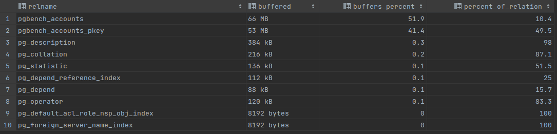
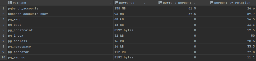
At the “a” picture we can see that accounts table and accounts_pkey table in total grab almost the whole shared buffer size, 119MB which is more than 92% of the whole shared buffer memory. In a column percent_of_relation it’s possible to see that it’s very important for the server to keep accounts_pkey table in memory, in spite of the accounts table which is buffered on 10.4%, this one is buffered on 49.5%. Having increased the shared buffer size to 256MB it’s possible to see at the “b” result, that accounts_pkey table is buffered on 89.7%.

‍

The second one query show usages count by relation:

‍-- usages count by relation
SELECT
c.relname, count(*) AS buffers,usagecount
FROM pg_class c
INNER JOIN pg_buffercache b
ON b.relfilenode = c.relfilenode
INNER JOIN pg_database d
ON (b.reldatabase = d.oid AND d.datname = current_database())
GROUP BY c.relname,usagecount
ORDER BY c.relname, usagecount;

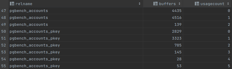
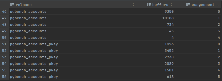
Usage count can tell a lot about shared buffer. If most of the relations have a small usage count like 0 or 1, probably it will be a good idea to increase a shared buffer size. After increasing the shared buffer size we can see in the picture “b” that there appeared more popular pages and there is better balance between low and high used relations. If we see a high accumulation of buffers with usage count it means that shared_buffer is optimized quite well and further increasing if its size will not lead to a better performance.

The same dataset was tested with the following command: ~$ pgbench -S -c 50 -t 25000 test_buffers; The result was:

• 128MB shared buffer ~ 140 ms connection time;
• 256MB shared buffer ~ 138 ms connection time;
• 1024MB shared buffer ~ 133 ms connection time;

WAL writer

WAL writer (Write Ahead Logging writer) is a mechanism that saves unstored data. All segments happening in the server are being recorded in the WAL segments anyway. Also he is responsible for:

• Recovery;
• Server startup;
• Replication.

Turning off the WAL writer (param. name: fsync) increases the DB performance especially on bulk operations, but leads to such problems as data inconsistency in case of power fail or crash.

The most important variables to setup are:

• max_wal_size - defines a soft limit for total WAL size;
• min_wal_size - defines a limit for minimal WAL size;

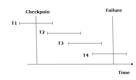
Checkpoints

Checkpoints are points in the sequence of transactions at which it is guaranteed that the data files have been updated with all information written before that checkpoint in a WAL sequence. At checkpoint time, all dirty shared buffer data pages are flushed to disk, marked as clean and a special checkpoint record is written to the log file.

It guarantees that on any crush all data before checkpoint will be saved

There are some variables, which using can improve the performance:

• checkpoint_flush_after - The default is 256kB (32 pages) on Linux, 0 elsewhere - saves data after defined number of pages;
• checkpoint_timeout - default is 5 min - saves data after some period of time;
• checkpoint_completion_target - default 0,9 - he specifies the target of checkpoint completion, he tells postgres how quickly he must finish checkpoint in each iteration.

It’s very easy to check WAL writer and checkpoints configuration:

‍-- Check WAL and checkpoints parameters
SELECT name, setting
FROM pg_settings
WHERE name LIKE '%wal_size%'
  OR name LIKE '%checkpoint%' ORDER BY name;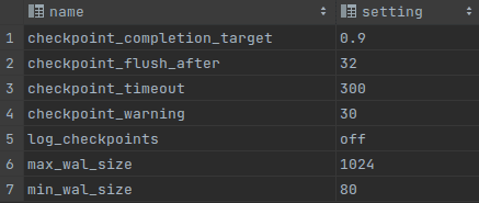

To improve the performance for Bulk data operations, it's necessary to increase the size of max_wal_size, checkpoint_flush_after, checkpoint_completion_target and checkpoint_timeout.

After increasing the value of such parameter like checkpoint_timeout from 5min to 20min, the number of disk I/O operations will be reduced, but operations themselves will take much more time. Decreasing the value will have the opposite effect.

Increasing the checkpoint time has one more impact. If DB has a lot of DML (INSERT / UPDATE / DELETE) queries and checkpoints occur very seldom, then there is a risk that the shared buffer will be filled up with data, which must be written or writing operations of huge amounts of data will affect other queries.

In most of cases postgres will tell us when some of those parameters must be changed It will be necessary to turn on (instruction the logging.

• LOG: checkpoints are occurring too frequently (9 seconds apart)
• HINT: Consider increasing the configuration parameter "max_wal_size".
• LOG: checkpoints are occurring too frequently (2 seconds apart)
• HINT: Consider increasing the configuration parameter "max_wal_size".

Cut from log the file

The background writer

He is running as a separate server process, his function is to issue writes of “dirty” (new or modified) shared buffers. When there is a lack of clean buffers, he takes some dirty ones and writes them into the files and marks those buffers as clean. Such an approach reduces the likelihood that server processes handling user queries will be unable to find clean buffers and have to write dirty buffers themselves. So, the main task is to let other processes go about their business instead of clearing the buffer when there are no clean pages.

A huge disadvantage is that the background writer causes a net overall increase in I/O load. In spite of checkpoints the background writer will write all repeatedly-dirtied pages.

• bgwriter_delay - 200ms by default - delay between writings;
• bgwriter_lru_maxpages - max. num. of buffers that will be written by process in each iteration

Vacuum

DB actually doesn't delete or update any rows on UPDATE or DELETE operations immediately. Those rows are only marked as deleted. The main task of vacuum is to mark such rows as being to reuse, and as a result tables take less disk space (free space mostly is not returned to the OS, but is going to be reused) and makes queries run faster.

‍

There are two types of vacuum, the first one is the autovacuum - does all described above and has next settings:

• autovaacuum_naptime - default 60s - checks if there is some work for autovacuum;
• autovacuum_max_workers - default 3 - max. autovacuum workers for one database;
• autovacuum_vacuum_threshold - default 50 tuples - the minimum number of updated or deleted tuples needed to trigger a vacuum in any one table;
• autovacuum_vacuum_scale_factor = default 0.2 (20%) - fraction of the table size to add to autovacuum_vacuum_threshold when deciding whether to trigger a VACUUM

‍

Example of vacuum:

‍-- Create a new table
CREATE TABLE vacuum_test (id int) WITH (autovacuum_enabled = off);
 
-- Insert data inside
INSERT INTO vacuum_test SELECT * FROM generate_series(1, 100000);
 
-- Check table size
SELECT pg_size_pretty(pg_relation_size('vacuum_test'));
 
--  Update each value
UPDATE vacuum_test SET id = id+1;
 
-- Check table size again
SELECT pg_size_pretty(pg_relation_size('vacuum_test'));
 
-- Vacuum the table
VACUUM vacuum_test;
 
-- Check table size again
SELECT pg_size_pretty(pg_relation_size('vacuum_test'));

As a result a free space will not be returned to the operating system and DB server will have some amount of free space, so in some amount of next operations DB will not request a new free space from the OS.

‍

The second type of vacuum cleaning is a VACUUM FULL. It rewrites data to new files, structures and reorders the table data and allows to return a free space to the operating system. It requires a special lock access to the table so it’s better to make VACUUM FULL when the server is used less of all. Also he takes a lot of time to run. The most important point why this kind of vacuum must be used is that he updates data statistics used by the planner. It allows a planner to be more effective. Also it’s useful to try VACUUM FULL when expected execution time is very different from the real one.

Parallelism

Parallelism allows running queries on several CPUs. The most useful is using parallelism for queries which collect data from many tables but return only several rows. Such queries can be 2 or even 4 times faster. Which query will run parallelly is defined by a planner.

• min_paralel_table_size - default 8 megabytes - minimal table size for parallel scan;
• max_paralel_workers_per_geather - max. number of parallel workers - will be never used for small tables. It's possible to set the max. numbers of parallel workers for exact one table;

Max number of parallel workers is limited by two variables:

• max_workers_processes - how many worker processes are available overall;
• max_paralel_workers - how many workers are available for parallel queries.

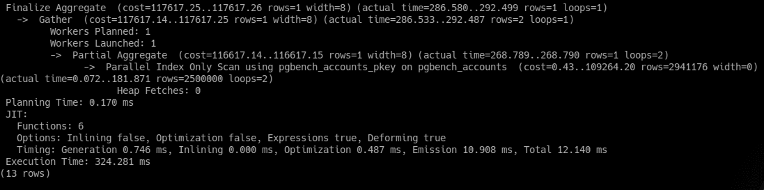
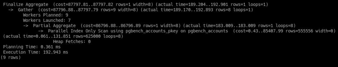
The execution time of such command as “EXPLAIN ANALYSE SELECT count(*) FROM pgbench_accounts;” with one parallel worker is more than 320ms, but seven ones as it’s possible to see in the picture below, it can be shorted to 192ms. Maximal number of parallel workers for the second example is ten, but there are only seven of them used, it’s because of the size of the table isn't large enough for using all ten workers.

Indexes

First of all, all indexes must be used only for columns with high cardinality (percent of unique values), for example an id column has 100% cardinality as each value is unique. By default postgresql adds a B-Tree index to the id column of each table.

‍

B-Tree indexes can handle equality and range queries on data that can be sorted into some ordering. A good idea is to use B-Tree for unique column for example with emails. But queries including patterns like this “col LIKE '%bar'.” will not be executed using indexes.

‍

PostgreSQL contains a lot of other indexes from HASH indexes which store data like a 32bit hash and can be used only in equality comparisons to SP-GIST indexes which support various kind of searches (for example “nearest-neighbor” ) and permits implementation of various data structures.

‍

PostgreSQL supports a lot of varieties of index scans. First of them is a common index scan which returns data according to the index. Another one is an index only scan; it means that needed data could be returned from the index file even without opening the table data file.

‍

In cases when the returned rows number is too little for sequential scan and too much for index scan postgresql uses a bitmap scan. It is a combination of sequential scan and index scan.

‍

A very good practice is indexing foreign keys. It’s very helpful in parent-child tables relationships, where the child table is bigger than the parent's one. Let’s create an orders table with 1 000 000 of rows, where each raw will have 4 items from items table:

‍-- Create orders table
CREATE TABLE orders (id SERIAL PRIMARY KEY, order_date DATE);
 
-- Create items table
CREATE TABLE items (
   id SERIAL NOT NULL,
   order_id SERIAL,
   name VARCHAR,
   description VARCHAR,
   created_at TIMESTAMP,
   CONSTRAINT fk_items FOREIGN KEY (order_id)
   REFERENCES orders(id));
 
-- Insert the data
WITH order_rows AS (
   INSERT INTO orders(id, order_date)
          SELECT generate_series(1, 1000000), now()
          RETURNING id
)
INSERT INTO items(id, order_id, name, description, created_at)
   SELECT generate_series(1, 4) id, o.id, 'product',
          repeat('the description', 10), now()
FROM order_rows AS o;
 
-- Make a select
EXPLAIN SELECT * FROM orders
JOIN items i on orders.id = i.order_id
WHERE orders.id = 666666;

The avg response time on DELL G15 running Kubuntu 22.04 was from 400ms to 600ms, but after creating an index on a foreign key column it decreased to 40-60ms for the same query:

‍-- Create and index of FK column
CREATE INDEX item_fk_index ON items(order_id);
 
-- Make a select
SELECT * FROM orders
JOIN items i on orders.id = i.order_id
WHERE orders.id = 666666;

Even with 25% cardinality the query execution is nearly 5 times faster. The same result was with 10% cardinality. Indexing foreign keys is very useful when we have tables with a huge amount of data in them, otherwise planner instead of an index scan will choose a sequential scan.

‍-- Cardinality check
SELECT (count(DISTINCT order_id)::FLOAT / count(*)) * 100 AS cardinality
FROM items;

In case, when we have a table with some kind of transactions but actively are used only not finished ones, we can create an index only for certain rows, for example for those where transaction status is not finished. One more benefit of such index is that he takes less disk space.

Usually indexes are used for fetching a small amount of data, but depending on frequency of queries and response time sometimes it will be reasonable to create an index from a column used by ORDER BY with LIMIT. ORDER BY by itself is a very hard command and requires a lot of time for its execution. In next case is shown the example, of using index together with ORDER BY:

‍-- Select data
EXPLAIN ANALYZE SELECT *
FROM orders
ORDER BY order_date DESC
LIMIT 25;
 
-- Create index
CREATE INDEX order_date_index ON orders(order_date);
 
-- Select data after creating index
EXPLAIN ANALYZE SELECT *
FROM orders
ORDER BY order_date DESC
LIMIT 25;

In spite of the fact that the cardinality of the order_date column is less than 1%, query execution is 2-4 times faster now. It’s thanks to the fact that data are already sorted in index file.

‍